How to hide or unhide rows & columns in Excel

Microsoft Excel’s Spreadsheets comes with hundred of features those are very useful to manage large amount of data in the rows and columns of this office program. Here are not going to its introduction as everybody know about Excel, instead, we will explain how to use hide and unhide rows or columns feature in Excel.

Now, where this feature would be useful, it solely depends on person why he or she wants to use rows or columns hiding feature of Excel, however, generally, if we don’t want to show some information to other or want to hide some data or figures, this will be handy. This tutorial work on almost all active or working versions of Microsoft Office Excel programs such as Excel 2007, 2010, 2016, 2017, 2019 or Office 365.

First, we see the process of hiding any rows or columns:

On this Page show

Hide or Unhide a complete Row in Excel

Open Microsoft Excel Software.
Import the Sheet which wants to use. If you already on that move to the next step.
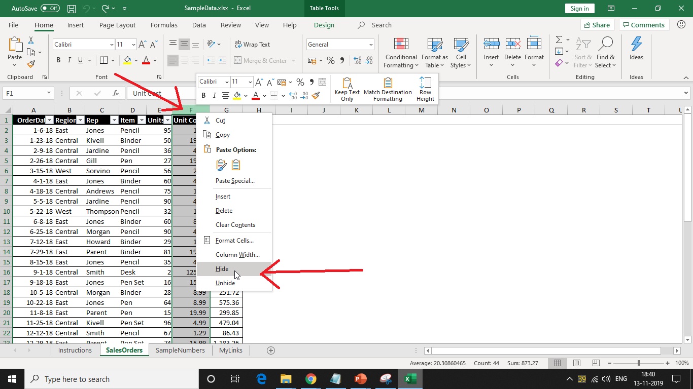
On your Excel to hide any complete row, go to it and right-click on top of it where the serial number series is given such as A, B, C, D and so on. See the screenshot for reference.
Now a pop-up menu will open, at the lower side you will find an option “Hide” select that. You can also use a keyboard shortcut to hide rows that is- Ctrl + 0 (zero). Just select the row and use it.
This will hide the selected complete row.
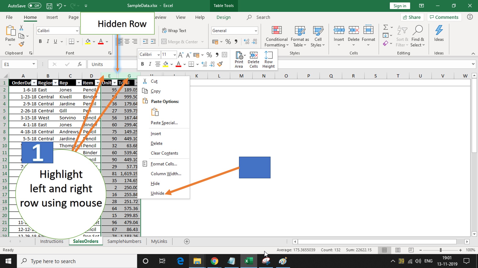
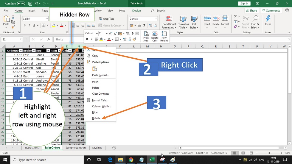
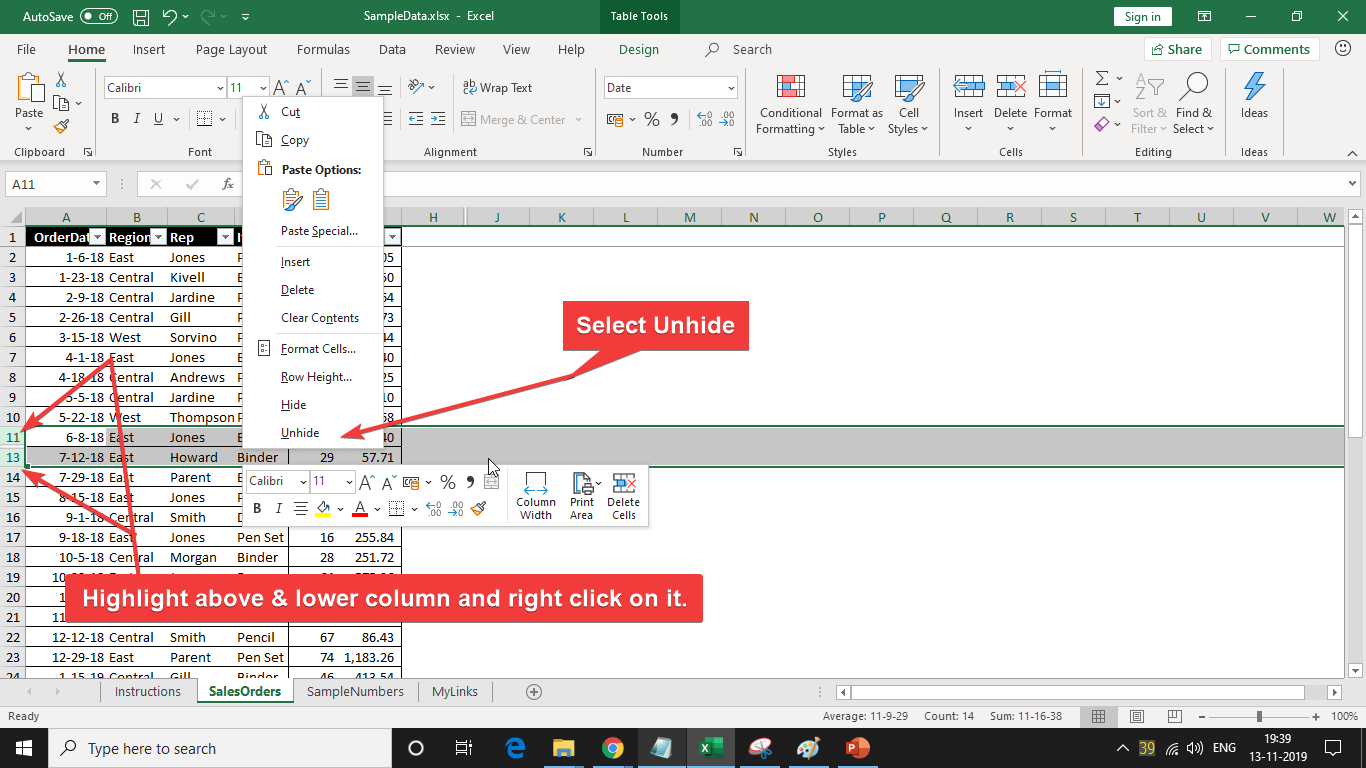
Now to unhide the row which you have hidden, use mouse pointer and highlight the left and right side of the hidden one and then right-click.
There you will see an option unhide, select that and you will get your row back.

See the Screenshots for more info:

Just right click on top of the row and select the Hide option. Ctrl+0 (zero) is a shortcut.

To unhide a row, use your mouse click on left row drag your mouse towards the right row of the hidden one. Now, right on it and select the unhide option. That’s it.

Hide or Unhide a complete Column in Excel

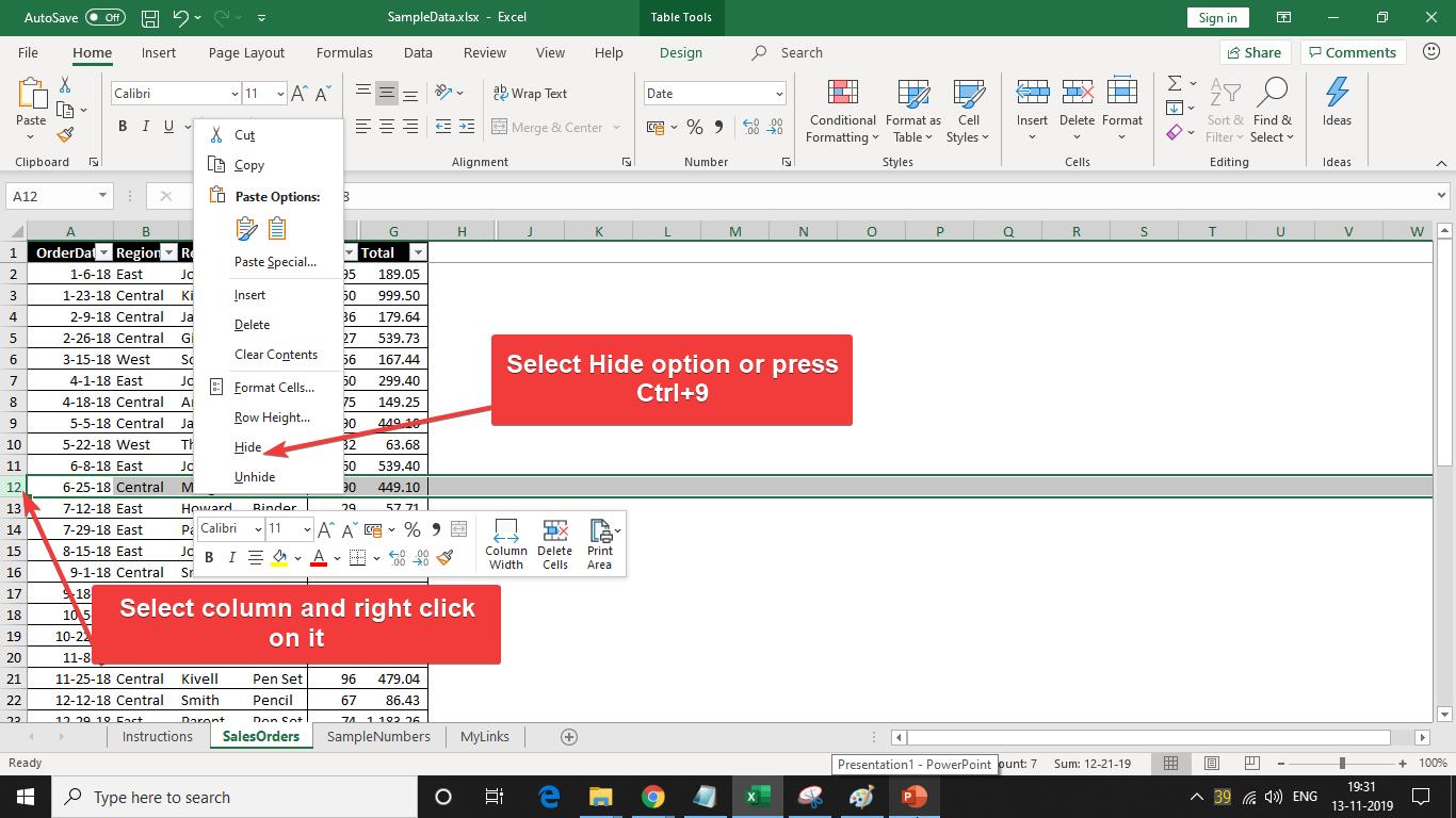
Go to the Excel sheet where you want to hide a column in Excel.
Select the entire column.
Right-click on it.
Select hide option or you can use shortcut key Ctrl+9 to hide the column.
To unhide just like we did for rows, select and highlight the upper and lower column of the hidden one and right to select unhide option. If you want to use a keyboard shortcut to unhide column then after highlighting press Ctrl+Shift+9.
For more info see the below two screenshots.

Hide entire column, select, right-click and hide.

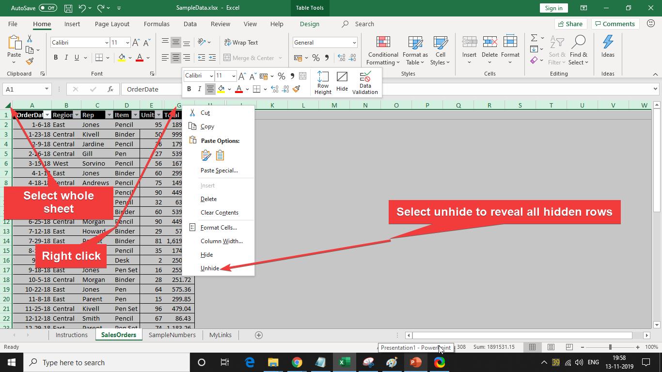
To unhide the entire column, highlight the upper and lower column, for example in the above screenshot we hid 12th number column and to get it back we use mouse pointer for highlighting above and lower ones and after that, we will right-click on it to select the unhide option or use keyboard shortcut Ctrl+Shift+9.

Unhide all columns and rows in excel

To unhide all hidden columns in any Excel sheets, go to the top left corner of your sheet area and click on + icon to select the whole sheet or alternatively you can use Ctrl+A shortcut. After that press, Ctrl+Shift+9 buttons simultaneously from the keyboard or just right-click anywhere on sheet and select unhide.

And for unhiding all rows at once, after selecting the whole sheet, right-click on the top area of the rows where the serial numbers are given (A, B, C..) and select unhide.